Learn Controls With Bobble-Bot (Part 1)

Posted on May 25, 2019 in tutorials

Feedback control is a fascinating subject that is crucial to the implementation of many modern smart devices including robotic systems. Lots of engineers shy away from the subject because the theory can be math intensive, the hardware and software can be expensive, and implementing controllers usually requires some level of comfort in computer programming. It is a challenge for instructors to incorporate a significant hands-on example in the classroom environment. This makes it difficult for students to gain an intuitive understanding of the subject.

To try to solve this problem, simulation tools are often used in place of real systems in order to help develop this intuition in a fraction of the time. This is one of the reasons Matlab Simulink is popular in controls classes at universities. Outside of the university environment, however, Matlab Simulink is costly. This makes it nearly impossible for hobbyists to experiment with the theory and the numerous online Matlab excercises that are posted to the web. Many are turning to platforms like the Arduino and Raspberry Pi to fill this gap.

Regardless of how you do it, if you want to get into robotics, I strongly advise that you spend a little time dedicated to gaining some familiarity with controls. Learn a little bit of the math theory, and practice the skill of programming (it's not that bad). You'll be glad you did because you'll have a better understanding of how robots really work.

This post will use Bobble-Bot as a platform for experimenting with feedback control at low cost. Bobble-Bot uses a combination of open-source simulation software and open-hardware in order to provide the user with a powerful set of tools for learning about feedback control. Let's jump right in and see how that's done.

Getting the simulator¶

Before we get too far, it's a good idea to go grab the Bobble-Bot simulation from here We will use the simulator to explore feedback control in an interactive way. Along the way, I'll show data from real test runs of an actual Bobble-Bot so that you can see how reality compares with the simulation. If you'd like to build or buy your own Bobble-Bot, head on over to SOE's website. The simulator is free and easy enough to use. To get started, follow the steps in the next section.

Building and running the simulation¶

The Bobble-Bot simulator requires ROS and Gazebo. Follow the instructions here and install ROS Melodic Desktop. Other recent versions of ROS should also work, but they are not officially supported at this time. The simulator also makes use of the Hector Gazebo plugins. Those can be installed using the command below.

apt-get install ros-melodic-hector-gazebo-plugins

Before starting the build process, make sure your ROS environment is active.

source /opt/ros/melodic/setup.bash

Get the simulation code and build it using catkin.

mkdir -p ~/bobble_workspace/src
cd ~/bobble_workspace/src
catkin_init_workspace
git clone https://github.com/super-owesome/bobble_controllers.git
git clone https://github.com/super-owesome/bobble_description.git

By now your bobble_workspace directory should look like so:

└── src
    ├── bobble_controllers
    │   ├── analysis
    │   ├── config
    │   ├── launch
    │   ├── src
    |   ...
    ├── bobble_description
    │   ├── imgs
    │   ├── launch
    │   ├── meshes
    │   └── xacro
    |   ...
    └── CMakeLists.txt

Build the Bobble-Bot simulation by running this command:

catkin_make
catkin_make install
source install/setup.bash

The Bobble-Bot controller package comes with a set of launch files that can be used to generate data from different runs of the simulation. As an example, the apply_impulse_force.launch file can be used to run the Bobble-Bot simulation and apply an impulse force in the X direction. This launch file accepts a few launch parameters. Most notably, the X component of the impulse force, and a flag to enable/disable the 3D graphics.

roslaunch bobble_controllers apply_impulse_force.launch \
impulse_force:=-1000 gui:=true

The launch file also instructs the simulation to log simulation data during the run. The data is placed in the following location by default:

ls ~/.ros | grep impulse_data
impulse_data.bag

You can override this default location like so:

roslaunch bobble_controllers apply_impulse_force.launch \
impulse_force:=-1000 gui:=true \
out_file:=~/bobble_workspace/src/bobble_controllers/analysis/impulse_test

To analyze what happened with the simulation run in more detail, run the commands below.

cd ~/bobble_workspace/src/bobble_controllers/analysis
python make_plots.py --run impulse_test.bag

The script above uses the analysis_tools Python module defined in bobble_controllers to load the simulation data and make the plots. After running the make_plots.py script above, you should see that two images were created: 'TiltControl.png' & 'VelocityControl.png'. They should look something like the following:

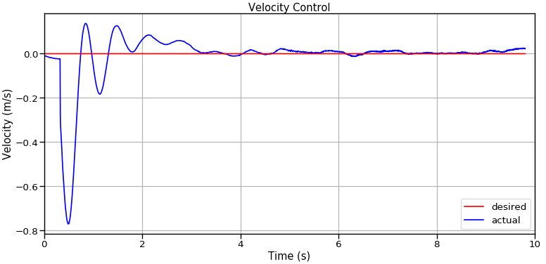
When working with feedback controllers, testing and analyzing your changes against an applied impulse force is often a good practice. Read this blog post series if you're interested in learning more about analyzing simulator data. The procedure outlined above should be sufficient for our needs in this series on feedback control. So, if you got everything running and were able to produce the plots above, then you are ready to proceed through the remainder of this tutorial series. Submit an issue on the bobble_controllers GitHub if you have any problems.

How does Bobble-Bot keep its balance?¶

Now that you've played around with the simulator a bit, let's start disecting how Bobble-Bot keeps its balance.

The gifs above show both the simulated and real Bobble-Bot's "impulse response". That's just another name for what happens when you give your system a little kick. Taking one look at Bobble-Bot is enough to see that it is a naturally unstable system. Without motors to control the wheels, Bobble-Bot would topple over almost immediately. In fact, that's intentional. Bobble-Bot was designed to be a real-life example of a classical textbook problem in control theory known as control of an inverted pendulum. This makes it an ideal system to show the connections between theory and practice. Let's start with just the bare essentials from linear control theory.

Feedback Control Basics¶

Feedback control is accomplished by the creation of a "feedback loop". The function of a feedback loop is to produce a desired output in response to changes in the state of a system as measured by sensors. The values of the system's state are measured by the sensors and then "fed back" to a control computer or control circuit.

Another name for the system and process under control is the "plant". In many cases, it is not possible or desirable to modify the internals of the plant and its process. Instead, engineers combine sensors and actuators with control computers to externally force the system to respond to a desired reference command.

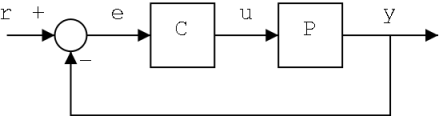
This entire approach is captured by the diagram above which depicts the basic structure of a feedback loop. These types of diagrams are known as block diagrams, and they are a very common way of capturing information about a controller design. Starting from the left, we have the reference command, r. The reference command represents a desired state for the system. This desired state is tracked as the output signal, y, of the plant process, P. The output signal is measured and "fed back" into the summation circle block. The feedback signal represents the current state of the plant output. The summation circle depicts that the error signal, e, is generated by subtracting the measured state from the desired state, r. Put simply, the error is the difference between what is desired and what has been measured. The feedback controller, C, processes the error signal and converts it to an output command, u. The output command is typically a command to an actuator which will cause a change in the plant process such that the state of the output signal approaches what was requested by the reference command. In this way, feedback controllers serve to drive a system to a desired state by eliminating the error between the reference command and a measured state.

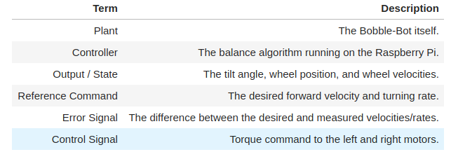
The diagram above captures a sort of general feedback controller design. It is a useful abstraction to help get familiar with some terminology that is common to all feedback controllers. Now that we know some the terminology and concepts, let's bring this abstract design down to something more concrete and relevant to our purposes. The table below summarizes the important parts of the block diagram above and how they are represented in Bobble-Bot's feedback loop.

PID Control¶

To get even more specific, Bobble-Bot's balance control algorithm relies on the principles of PID control. PID controllers are a specific class of linear feedback controllers that require tuning three separate gains (controller constants that effect performance). With PID control, the engineer must settle upon values for a proportional, integral, and derivative gain. The block diagram below shows the inside of a PID controller.

While the above diagram is instructive, it might imply a complex implementation. In reality, a basic PID controller is very easy to implement in software. The couple of lines below implement a PD controller fairly well and can take a you surprisingly long way.

error_dot = error - last_error // finite difference with dt captured within Kd
control_cmd = error * Kp + error_dot * Kd
last_error = error

Integrators add some subtle complexities that I won't go into right now. The complexity comes from the fact that a real system will have to deal with integral windup. The challenge with PID in practice comes down to determining the values of the three gains. This is often done by a sort of intelligent guess and check approach. In order to guess and check intelligently, however, you have to understand how each gain effects the output signal.

The Kp term is known as the proportional gain. It adds to the output signal a value that is proportional to the error signal times the gain's value. If the error is large and positive, the control output will be proportionately large and positive.
The Ki term accounts for past values of the error by continually summing up the error signal each time the controller runs. If there is a remaining error after applying the proportional gain, the integral term will work to eliminate it as it will grow as long as any error remains. The integral term is the way to ensure that the plant eventually reaches the desired state without any lingering error.
The Kd term accounts for changes in the error signal. If the error is rapidly changing the Kd term can help dampen the effect. The derivative term helps to reduce oscillations and system vibrations. It can be thought of adding stiffness to the system.

Here's a gif of how the PID tuning process typically effects the output signal when the reference command is a step function.

Let's apply some of this new found knowledge to a simple approximation of Bobble-Bot: the cart-pendulum system.

An Example: The Cart Pendulum Plant Model¶

The cart-pendulum system is a form of an inverted pendulum that consists of a mass at the end of a massless rod that is attached by a rotational pin joint to a movable cart. This system is shown in the figure below. The inverted pendulum on top of the cart is in an unstable equilibrium when it is standing upright. Theoretically, this equilibrium can be maintained without active control as long as there are no disturbance forces acting on the system. Clearly such conditions do not exist in reality. The real system can be kept in balance by using a force based feedback controller. This controller applies a force to move the pendulum’s center of gravity (CG) in such a way that it dampens the resulting motion. The force is actively controlled based on sensor feedback in order to bring the system back to its natural unstable equilibrium. The system is analogous to a person balancing a broom in their hand.

The equations that describe this system are given below.

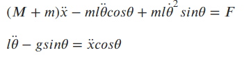
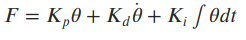
The above two equations describe the dynamics of the cart-pendulum system. These differential equations model the plant motion, and they are sometimes referred to as a "plant model". The Bobble-Bot simulation can be thought of a plant model as well. Assuming we can measure and feed back theta and theta dot, we can design a PID control algorithm that generates a force to keep the pendulum balanced. Here's the PID control law that we could use.

Controlling the Cart Pendulum¶

Evan Boldt wrote a great little web simulator of this system and the control law discussed above. The simulator makes it easy to practice PID tuning. Click on the image below to launch the simulator. I highly recommend using his sim to apply what you learned in the previous sections. See if you can stablize the pendulum by tuning the control gains. If you can do that, you will be well on your way for the Bobble-Bot balance tuning to come in part 2 of this series.

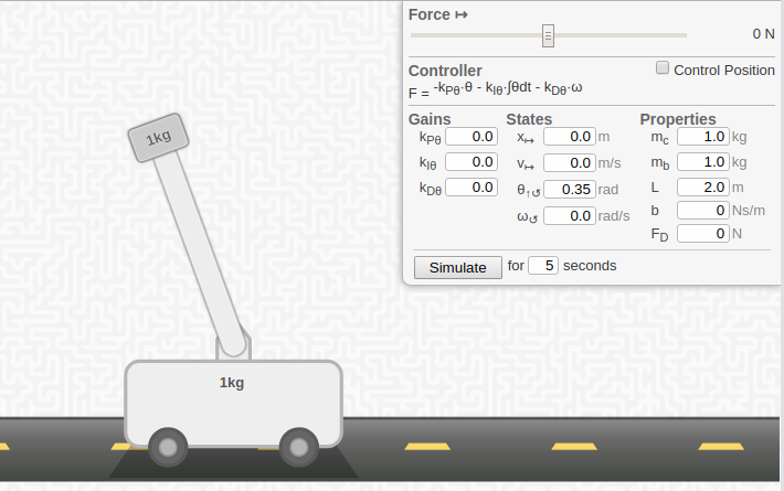
Evan also has a nice PID tutorial to go along with his simulator. Thanks Evan!

Next Steps¶

That concludes part one of this series. We've really just scratched the surface of linear control theory. Hopefully it has been enough to whet your appetite. Read the references below if you'd like to dig deeper. In part two, we'll apply what we've learned in this post in order to understand and tune Bobble-Bot's tilt controller. We'll use the simulator to do this, but I'll also present real Bobble-Bot data for comparison. It should be fun, so when you're ready, proceed on to part two.

References¶

Special thanks to the author's of all the content below.