BobbleSim

In part 1 we looked at how to generate data for the Bobble-Bot simulator. Either go back and read that post, or download the data here and keep reading. With your data ready, we can begin our analysis using Jupyter Notebook. First, let's get our analysis environment setup.

All of the dependencies can be installed using pip.

sudo apt-get install python-pip python-dev build-essential
pip install pandas jupyter rosbag_pandas seaborn

Let's use the sample analysis script provided in the bobble_controllers repository to test that we now have the needed packages.

cd ~/bobble_workspace
catkin build
source devel/setup.bash
cd ~/src/bobble_controllers/analysis
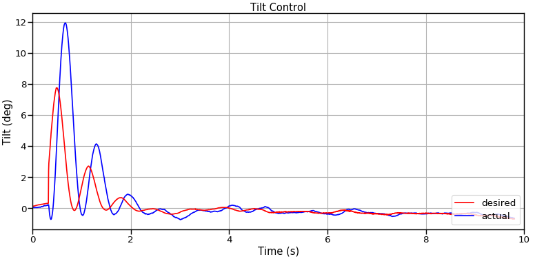
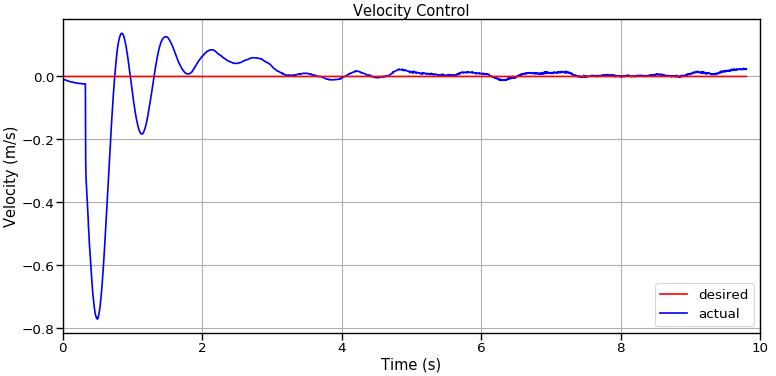
python make_plots.py -r impulse_force.bag

If all went well a TiltControl.png and VelocityControl.png file will be created in the working directory. These plots should look like this:

Tilt Control

Velocity Control

The analysis script can be used to make these two plots for any of the runs (including the data you produced in part 1). Here's how to use it:

python make_plots.py --help
usage: make_plots.py [-h] [-r RUN] [-o OUT]

optional arguments:
  -h, --help         show this help message and exit
  -r RUN, --run RUN  Bag file for simulation run of interest
  -o OUT, --out OUT  Output directory.

Using the analysis_tools module¶

The make_plots Python script provides a good introduction to making plots of ROS data using Pandas and Matplotlib. For your convenience, the bobble_controllers repository provides a helper Python module to facilitate making plots of the Bobble-Bot simulation data. The analysis_tools module is written to be fairly generic so that it can be adapted to more general ROS data analysis. Check it out, and feel free to adapt it to your own project.

Our simulation data is stored in ROS bag format. Pandas DataFrames are a more convenient data representation for a Python+Jupyter based analysis. Our bag files can be quickly converted to this format by making use of the provided analysis_tools.parsing module. This article discusses how the parsing module loads a ROS bag file into Pandas in more detail. Here's the relevant snippet of code that loads the simulation's bag file into a Pandas DataFrame.

from analysis_tools.parsing import parse_single_run
print "Loading sim data from run : " + str(run_name) + " ... "
df = {}
df[run_name] = parse_single_run(sim_data_bag_file)

Of course, this post is about a Jupyter Notebook based analysis. Let's see how we can use the analysis_tools module to load data into a notebook.

Loading data into Jupyter¶

The first step is to activate your environment and load Jupyter Notebook. To help you follow along, the Jupyter Notebooks for this series can be found here.

cd ~/bobble_workspace
source devel/setup.bash
jupyter

With Jupyter now open, navigate to the folder containing your data and .ipynb file. In that folder, you will also find a file called nb_env.py. This file is used to import the needed modules and load all the bag files found in the data directory. Feel free to replace the contents of the data directory with the simulation data you generated from part 1. To load this file and view the simulation runs available for analysis, use the cell shown below.

In [26]:

# Load anaylsis environment file. This file defines data directories
# and imports all needed Python packages for this notebook.
exec(open("nb_env.py").read())
# Print out the df dictionary keys (the test run names)
df.keys()

Reading all bag files in directory : 
/home/mike/blogs/mike-moore/content/notebooks/ros-jup-analysis/data
Successfully loaded runs :

Out[26]:

['impulse_force', 'drive_square_js_response', 'balance', 'no_balance']

We now have all the data from the simulation runs generated in part 1. Let's use Pandas to demonstrate some basic manipulation of the simulation data.

Print sim data in tabular form¶

We can print the first five rows from the 'balance' run in a nice tabular form like so:

In [27]:

n_rows = 5
df['balance'].loc[:, 'Tilt':'TurnRate'].head(n_rows)

Out[27]:

	Tilt	TiltEffort	TiltRate	TurnRate
time
0.000	0.012409	0.0	-1.548588	0.006942
0.005	0.001358	0.0	0.459353	0.474901
0.010	-0.001004	0.0	1.230456	1.599712
0.015	-0.005767	0.0	-0.108348	1.204383
0.020	0.003489	0.0	0.379041	-0.893774

Search for a column¶

Here's how to search for a column(s) in a DataFrame:

In [28]:

search_string = 'Vel'
found_data = df['no_balance'].filter(regex=search_string)
found_data.head()

Out[28]:

	DesiredVelocity	ForwardVelocity	LeftMotorVelocity	RightMotorVelocity
time
0.000	0.0	-0.000003	-0.002918	-0.002919
0.005	0.0	-0.000003	-0.002918	-0.002919
0.010	0.0	-0.000003	-0.002918	-0.002919
0.015	0.0	-0.000003	-0.002918	-0.002919
0.020	0.0	-0.000003	-0.003891	-0.003891

Get all column names¶

You can view all of the data available in a given run like so:

In [29]:

df['balance'].dtypes.index

Out[29]:

Index([u'ControlMode', u'DesiredTilt', u'DesiredTurnRate', u'DesiredVelocity',
       u'ForwardVelocity', u'Heading', u'HeadingEffort', u'LeftMotorEffortCmd',
       u'LeftMotorPosition', u'LeftMotorVelocity', u'MeasuredTiltDot',
       u'MeasuredTurnRate', u'RightMotorEffortCmd', u'RightMotorPosition',
       u'RightMotorVelocity', u'Tilt', u'TiltEffort', u'TiltRate', u'TurnRate',
       u'time'],
      dtype='object')

Find the maximum value of a column¶

In [30]:

print "Max tilt no_balance run: %0.2f " % df['no_balance']['Tilt'].max()
print "Max tilt balance run: %0.2f " % df['balance']['Tilt'].max()

Max tilt no_balance run: 89.70 
Max tilt balance run: 2.88

Many more data processing and manipulation functions are possible. Consult the Pandas documentation for more information.

What's Next?¶

This post has demonstrated how to make a few plots of our simulation data from the command line. It also covered how to load the simulation runs into Jupyter Notebook. Finally, we explored using various Pandas functions to manipulate and print out this data within Jupyter. In part 3, we will show how to post process this data using NumPy, and then make some plots that capture the Bobble-Bot balance controller's performance.