This post relies on lessons learned in part one and part two of this three part series on analyzing ROS data using Jupyter Notebook. If you haven't read parts one and two, I highly recommend checking those out before continuing on. In the final part of this series, we will examine data from the test runs performed in part one. Our end goal is to analyze the performance of Bobble-Bot's balance controller during the drive square test shown below.

Before we get ahead of ourselves, let's load our analysis environment so that we can access our data using Pandas.

Plots in Jupyter Notebook¶

Let's start by opening up the Jupyter Notebook for part three found here. We ended part two after succesfully loading in the simulation data from our four test runs. We stopped just short of making plots within Jupyter Notebook. Let's pick up where we left off by creating a plot of the tilt angle during the balanced and un-balanced runs. This will allow us to investigate a modular strategy for creating plots of this data within Jupyter. This approach will allow us to create many different plots of interest with just a few lines of Python code. It will serve us well as the analysis ramps up in complexity.

Understanding plots.yaml¶

In the folder containing the notebook, you will find a file called plots.yaml. Go ahead and open that file up in your favorite text editor and examine its contents. Here's a snippet from that file:

measured_tilt:
  title : 'Tilt Angle'
  y_var: 'Tilt'
  x_label: 'Time (s)'
  y_label: 'Tilt (deg)'
  runs : ['no_balance', 'impulse_force']
  colors : ['grey', 'orange']
  linestyles: ['-' , '-']
  legend:
     no balance:
       color: 'grey'
       linestyle: '-'
     balanced:
       color: 'orange'
       linestyle: '-'
  xlim: [0.0, 10.0]

If you have never seen YAML before, this file may seem a little mysterious. YAML stands for YAML Ain't Markup Language. It's a configuration format that is commonly used for creating configuration objects. YAML is used extensively within the ROS ecosystem. In fact, the Bobble-Bot balance controller is also configured using YAML. YAML allows you to encode an object within a human readable file format. There are many open-source libraries that will parse this format and create an object representation in your language of choice. For our analysis, we will rely on PyYAML to read our plots.yaml file.

Using PyYAML to read this file is simple. The cell below loads in the plotting configuration file used for this analysis.

The parse_config_file function handles the call into PyYAML in order load our plotting configuration objects. These configuration objects hold important values, strings, and dictionaries that we will make use of when rendering a plot. Let's take a look at what is contained within the pc object returned by the parse_config_file function.

We see that pc contains a Python dictionary that maps a plot name to a plot configuration object (another Python dictionary). For example, if we want to print out the name of the variable to be plotted on the y-axis for the measured_tilt plot we can do the following:

Futhermore, if we want to create a copy of a plot configuration object, we can do the following:

Creating copies of plot configuration objects is useful when you would like to create a new plot that's very similar to the template one specified in plots.yaml. In this way, we can quickly create a new plot configuration object that will inherit all the properties from the one specified in plots.yaml. However, we can tailor the copy to meet the needs of our specific plot. As an example, let's use the analysis_tools.plots module to quickly render two plots of the same information for two different runs of the simulation. First, let's create two plot configuration objects, one for each plot.

Notice how we can also create copies of copies...nice! Next, let's render these plots using the make_static_plot function found in the analysis_tools.plots module:

We can even use the same measured_tilt configuration object to co-plot both runs on the same plot:

Hopefully the examples above have illustrated how to use plots.yaml and the associated configuration objects to make all kinds of different plots. The great thing about doing your analysis in a Jupyter Notebook is that the whole process is interactive. Try creating your own plots by inserting some more cells into your notebook. I will show some more examples in the sections to follow.

Post-Processing simulation data with NumPy¶

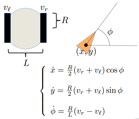
Currently, Bobble-Bot does not track its x,y world position internally because it is not needed by the balance controller. For this analysis, we will want to look at some commanded trajectories in world coordinates. In order to do this, we must post-process the simulation data. To compute the position in world coordinates, we can use a kinematic model for a differential drive robot. The model to be used is described in the graphic below. Special thanks to Professor Magnus Egerstedt at Georgia Tech.

The Python code below defines a function that uses this model in order to compute x, y position and velocity in world coordinates for each test run. The function relies on both SciPy and NumPy for some of the math operations.

Let's loop over all our runs and call this function so that we have this position data for each data set.

Analyzing the impulse force test¶

Our data is now ready for further analysis. Let's start with a simple case, the impulse force test. This is a useful test for evaluating the balance controller as it allows us to look at how the controller responds to an applied impulse force. Let's look at the tilt and velocity control performance after the impulse is applied.

This plot shows what you would expect for an impulse force applied in the -X direction. During this test the robot is in the balance mode. In this mode, the robot is trying to hold zero velocity. The applied impulse causes the robot to quickly accelerate in the -X direction. The job of the velocity controller is to reject this impulse by controlling the velocity back to zero. The plot above shows that the velocity controller is able to achieve its goal. In order to reject the -X disturbance force, the velocity controller modulates the desired tilt. In response to the -X impulse, the velocity controller commands the robot to tilt forward. The tilt controller then commands torque to each motor to achieve this tilt angle. This tilting motion serves to simultaneously control the velocity and reject the disturbance. Let's look at the tilt response to see this in action.

Here we see the velocity controller commanding a positive tilt to the tilt controller (red line) in response to the -X impulse. In response to this forward tilt, the tilt controller successfully tilts the robot forward. This tilting motion causes the robot to begin to accelerate back in the +X direction. The velocity controller detects this change in velocity and begins to ramp down the forward tilt command until it is zero. This tilting motion brings the robot back to its balanced and rested state. The balance controller has successfully used its velocity and tilt controllers simultaneously to reject the impulse force and remain standing.

Analyzing the Balance Test¶

This section will look at the data from the balance test in more detail. This test lasts about thirty seconds. During the test, the robot is commanded to drive forward and then backward. After those commands are executed, the robot is commanded to turn right and then back to the left. Let's make some plots to confirm the robot performs as expected.

Commands vs Response¶

Using the velocity control plot as our template, we make some slight modifications to use the balance run and limit the x axis to between 0 and 35 seconds. The plot below should show the velocity being commanded to 0.1 m/s, -0.1 m/s, and back to rest. We expect the robot to respond to these commands appropriately with some tolerance for noise and error in the state.

In order to drive forward and backward, Bobble-Bot's velocity controller commands a positive and then negative tilt to the tilt controller. The effort sent to each motor in order to track this tilt command causes the robot to drive forward and then backward. We can confirm this behavior by analyzing the tilt controller performance.

The plots above confirm the velocity and tilt control performance during the balance test. Let's now look at the turning commands that were sent during the test.

This concludes our analysis of the balance test. The last test to look at is the drive square test.

Analyzing the Drive Square Test¶

The drive square test is performed by issuing a canned set of joystick commands to drive Bobble-Bot in a square. These commands were generated by manually driving the robot during a simulation run and logging the joystick command data using rosbag record. The previous sections have served to validate the velocity, tilt, and turning controller. This final plot will show all of these controllers working together to track a commanded trajectory. The plot below shows the commanded position in X,Y world coordinates versus the actual X,Y position.

Bobble-Bot's balance controller seems to be working as expected!

Conclusion¶

Hopefully this post has provided a good introduction to using Jupyter Notebook for ROS robots. Keep in mind, Jupyter is not limited to ROS applications. It can be used in a wide variety of analysis and data science applications. Jupyter notebooks give others a chance to reproduce your results. They are meant to be shared with others so that they can interact with your work and check or extend your results. In that spirit, you can find the Jupyter Notebooks that were used to create this blog post series here.

This post concludes the three part series on using Jupyter to analyze ROS data. As always, feel free to contact me or leave a question in the discussion section below. Thanks for reading!